Policy Gradient Demystified
This is a simple explanation of Policy Gradient algorithm in Reinforcement Learning (RL). First, some background of Supervised Learning is presented and then, Policy Gradient method is studied as an extension to the Supervised Learning formulation. The blog post will clarify some of the notations usually covered in Reinforcement Learning lectures and build the basics for studying advanced RL algorithms.
Supervised Learning Background
Let us start with a simple MultiLayer Perceptron (MLP) which is built for the task of classification. In a typical MLP, we have \(C\) output units, where \(C\) is the number of classes in the classification problem and we train it with cross entropy loss. The cross entropy between the prediction \(\mathbf{\hat{y}}\) (\(\mathbf{\hat{y}}\) is a \({C \times 1 }\) vector) and ground truth label \(\mathbf{y}\) (which is usually one-hot) is given by:
If we have \(N\) training samples, then the cross entropy loss over the samples will be \(\sum_{i=1}^{N} H(\mathbf{\hat{y}}_i, \mathbf{y}_i)\).
The above formulation can also be viewed from a different perspective. If we have \(N\) observed variables \(y_1 \dots y_n\) (ground truth labels for the data samples) and a function approximator (say MLP) with parameters \(\theta\), then likelihood \(lik(\theta)\) is defined as:
\(p(y_i | x_i, \theta)\) gives the probability estimated by our model with parameters \(\theta\) for the observed variable \(y_i\), given the input \(x_i\). In layman terms, if we are using neural networks, we calculate likelihood function by multiplying the probability at the corresponding \(j_i\) output unit (where \(j_i\) is the ground truth label of the data sample \(i\)) for each input sample \(x_i\). By maximizing the above likelihood function, we find the parameters \(\theta\) which make the observed data “most probable”. In practice, rather than maximizing the direct likelihood, we usually minimize the negative log likelihood function which is much easier to deal with mathematically:
Thus, Supervised Learning problem for the task of classification can be formulated as:
Minimize \(-\sum_{i=1}^{N} \log(p(y_i | x_i, \theta))\)
\(= -\sum_{i=1}^{N} \log(\hat{y_i}^{j_i})\) (\(j_i\) is the actual class of sample \(i\) and \(\hat{y_i}^{j_i}\) refers to the probability estimated by MLP)
\(= -\sum_{i=1}^{N} \sum_{j=1}^{C} y_i^{j_i} \log(\hat{y_i}^{j_i})\) (since \(\mathbf{y}_i\) is a one hot vector with class \(j_i\), we can replace \(\hat{y_i}^{j_i}\) with summation)
\(= \sum_{i=1}^{N} H(\mathbf{\hat{y}}_i, \mathbf{y}_i)\)
We have proved that minimizing the cross entropy loss \(\sum_{i=1}^{N} H(\mathbf{\hat{y}}_i, \mathbf{y}_i)\) is equivalent to minimizing the negative log likelihood \(-\sum_{i=1}^{N} \log(p(y_i | x_i, \theta))\).
Introduction to Policy Gradient
In Monte Carlo techniques of Reinforcement Learning, we train our agent in episodic manner which means we run it in an environment (which is usually a game) till termination and just based on the outcome (win or loss) of the run or episode, we optimize our actions. Each time step of the episode is called a state and the goal of Reinforcement Learning is to find optimal action for each state. Note that we can’t train the agent in supervised fashion because we would need the correct action label for each state which we don’t have.
In Policy Gradient, we first run our agent for an episode and observe the reward at the end. If we win, the reward is positive and we encourage all the actions of that episode by minimizing the negative log likelihood between the actions we took and the network probabilities. If we lose, we do the opposite: discourage the actions we took in an episode by maximizing the negative log likelihood. By doing these updates repeatedly for several episodes, we hope that our network will learn the optimal policy (“policy” in RL literature refers to the mapping from state to action). For the minimization or maximization of likelihood based on reward, we tweak the log likelihood formulation of Supervised Learning by adding an extra term called “advantage” \(A_i\):
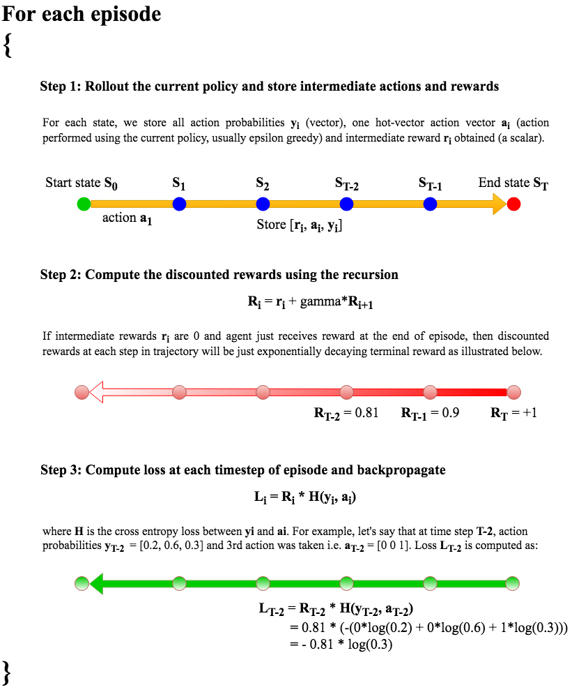
\(A_i\) could be +1 or -1 based on the outcome of the episode. However, the +1/-1 advantage function would penalize all the actions in an episode equally which is probably not optimal. We do something better here by making an assumption. The assumption is that the effect of current action will decay exponentially over time. We thus replace \(A_i\) with the discounted rewards. The following figure illustrates the complete Policy Gradient algorithm.
There are more advanced versions of this naive Policy Gradient algorithm like baseline, actor-critic etc. which tweak the advantage function \(A_i\) in a smarter way and improve the convergence and sample efficiency.
The PyTorch implementation of the naive Policy Gradient algorithm discussed in this blog post for the OpenAI Gym Cartpole-v0 environment can be found here.